Optimizing Industrial Equipment Maintenance Schedule Intervals

Determining precise industrial equipment maintenance schedule intervals requires moving beyond arbitrary calendar-based routines and OEM default recommendations. Default intervals are typically calculated for ideal operating conditions, which rarely match the thermal, mechanical, and environmental realities of a specific production floor. To optimize asset uptime and minimize total cost of ownership, maintenance engineers must apply statistical failure modeling, condition-based thresholds, and precise P-F interval calculations.

The Mathematics of Failure: Weibull Distribution Analysis

Fixed-time preventive maintenance (PM) is only mathematically justified when equipment exhibits a wear-out failure mode. This is determined using the Weibull distribution, specifically the shape parameter (β). According to reliability data exchange standards like ISO 14224:2016, collecting accurate failure data is the prerequisite for this analysis.

• β < 1.0 (Infant Mortality): The failure rate decreases over time. Performing scheduled maintenance actually increases the probability of failure due to human error during reassembly or introduction of contaminants. Action: Run-to-failure or condition monitoring only.
• β = 1.0 (Random Failures): The failure rate is constant. Age-based intervals are useless. Action: Implement redundancy or continuous IoT condition monitoring.
• β > 1.0 (Wear-Out): The failure rate increases with time. This is the only scenario where fixed industrial equipment maintenance schedule intervals are effective. Action: Calculate the interval just prior to the steep ascent of the failure curve.

Engineering Insight: If your CMMS data shows a Weibull β of 0.8 for a specific CNC spindle bearing, extending the PM interval or switching to vibration-based monitoring will immediately reduce your overall failure rate by eliminating maintenance-induced infant mortality.

The P-F Curve and Inspection Frequencies

When condition-based maintenance is selected, the inspection interval must be derived from the P-F interval. The P-F interval is the elapsed time between a Potential failure (P) — the point where a defect is first detectable via ultrasound, thermography, or vibration analysis — and a Functional failure (F) — the point where the machine can no longer perform its required function.

The industry-standard rule of thumb is to set the inspection interval at P-F / 2. However, for critical assets where the cost of unplanned downtime exceeds $10,000 per hour, engineers should target P-F / 3 or P-F / 4 to account for false negatives and sensor drift. For example, if ultrasonic analysis detects a bearing defect 8 weeks before catastrophic seizure (P-F = 8 weeks), the inspection interval must be set to 4 weeks maximum, or 2 weeks for critical path machinery.

Technical Baselines by Equipment Class

While condition monitoring is superior, baseline time-based intervals are still required for consumable replacements and fluid degradation where continuous sensors are cost-prohibitive. The following table outlines highly specific baseline intervals derived from heavy-industry operational averages.

Equipment Class	Component / Fluid	Baseline Interval	Technical Specification / Action
Hydraulic Power Units	Hydraulic Fluid (Group II)	4,000 Hours	Replace if ISO 4406 cleanliness exceeds 18/16/13 or TAN > 2.0 mg KOH/g.
Rotary Screw Compressors	Airend Bearings	40,000 Hours	Complete rebuild. Use synthetic PAO lubricants to prevent varnish buildup.
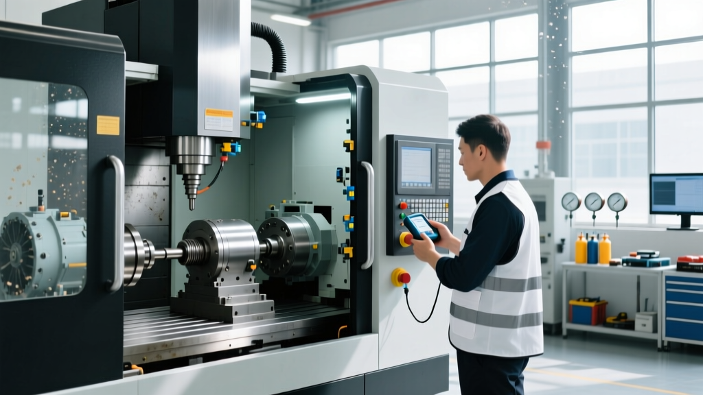
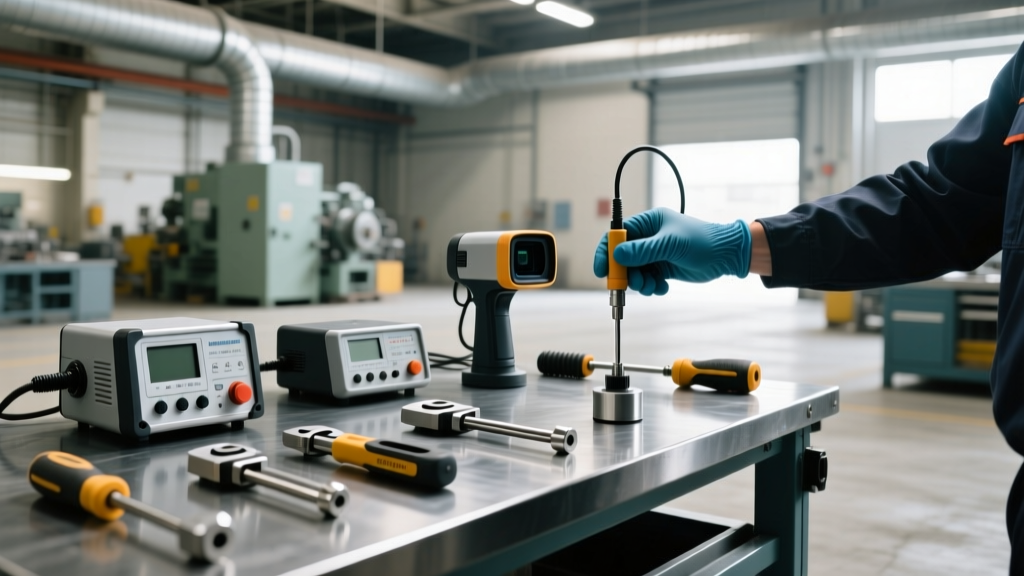
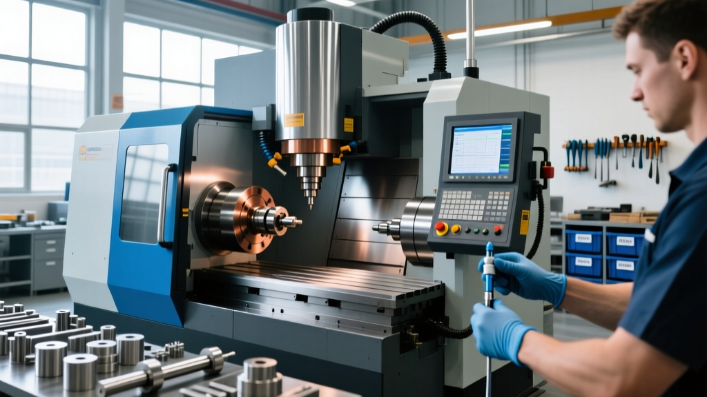
CNC Machining Centers	Spindle Drawbar Force	6 Months	Verify retention force remains > 2,500 lbs (11 kN) using a calibrated force gauge.
Overhead Bridge Cranes	Hoist Wire Rope	12 Months / 2k Cycles	Magnetic flux leakage (MFL) testing per ASME B30.2 standards.

Condition-Based Modifiers: Integrating ISO Vibration Standards

Modern interval optimization relies heavily on edge-computed vibration data. Rather than scheduling a teardown based on runtime hours, maintenance triggers are tied to specific velocity thresholds defined in ISO 20816-1:2016 (which supersedes ISO 10816). For standard industrial machines (Group 2, 15 kW to 300 kW), the intervals are dynamically adjusted based on the following RMS velocity readings:

Zone A: Good

< 2.8 mm/s RMS
Standard OEM baseline intervals apply. No action required.

Zone B: Satisfactory

2.8 to 4.5 mm/s RMS
Reduce inspection intervals by 50%. Schedule oil debris analysis.

Zone C: Unsatisfactory

4.5 to 7.1 mm/s RMS
Immediate work order generation. Machine must be scheduled for downtime within 14 days.

By programming your SCADA or IIoT platform to automatically trigger CMMS work orders when a 7-day rolling average crosses from Zone A into Zone B, you transition from rigid calendar intervals to dynamic, need-based intervals. This prevents both premature teardowns and catastrophic seizures.

Step-by-Step Framework: Deriving Custom Intervals

To establish a mathematically sound maintenance program for a newly commissioned production line, follow this sequential framework:

1. Define the Functional Failure Limit: Determine the exact metric at which the machine fails its purpose (e.g., a pump failing to deliver 500 GPM at 40 PSI, or a motor exceeding 85°C stator temperature).
2. Identify Detectable Degradation Signals: Map the P-F curve. Can you detect cavitation via ultrasound before flow drops? Can you detect misalignment via phase-angle vibration before bearing temperature spikes?
3. Calculate the Baseline P-F Interval: Use historical CMMS data or OEM preventive maintenance guidelines to estimate the time from first detectable signal to functional failure.
4. Apply the Criticality Multiplier: If the asset is a bottleneck (criticality score 9-10), divide the P-F interval by 3. If it is non-critical with redundancy (score 1-3), divide by 1.5 or utilize run-to-failure.
5. Implement and Refine via Weibull: After 18 months of operation, extract the failure and suspension data. Plot the Weibull distribution. If β is less than 1, your PM tasks are introducing defects; eliminate them and rely solely on the condition-based triggers established in Step 2.

Optimizing maintenance intervals is not a one-time configuration task. It is a continuous feedback loop requiring rigorous data collection, statistical validation, and alignment with real-time sensor telemetry. Facilities that enforce dynamic, data-backed intervals consistently realize a 20% to 30% reduction in maintenance labor costs while simultaneously increasing overall equipment effectiveness (OEE).